View Modes

HEXRDGUI includes various ways to visualize detector data, including a raw view and several different projections (Cartesian, Polar, and Stereo).

The type of view is switched by simply clicking on the corresponding tab in the "Image Mode" widget, which is by default on the right of the application.

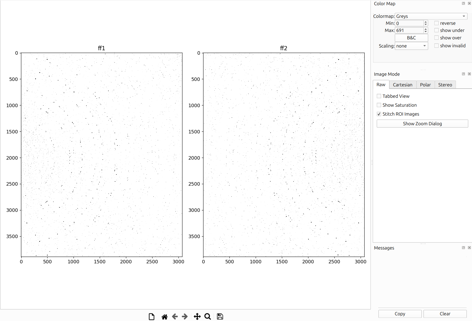
Raw View

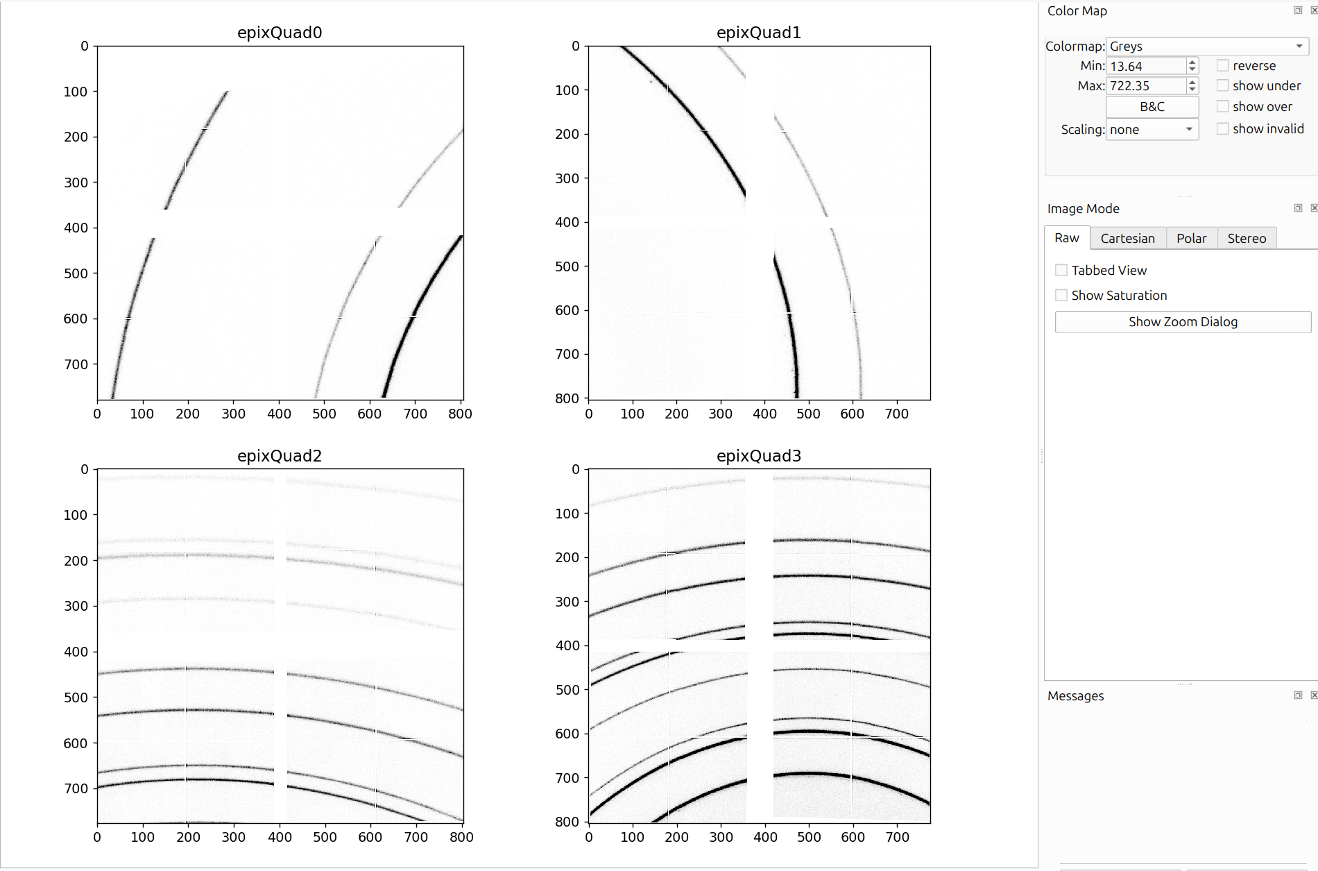
The raw view is a basic view of all detector images loaded in. If there is more than one image, the detector images will by default be displayed in two columns.

Raw View Options

The following options are available in the Image Mode panel for the raw view:

• Tabbed View: Display each detector image in a separate tab rather than side by side.
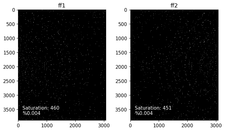
• Show Saturation: Displays the number and percentage of pixels at or above the detector's saturation level as text on each detector image, like so:

• Stitch ROI Images: Stitch subpanel images into larger detector images (see Stitching Raw Images below). This option only appears if an instrument with subpanels is loaded.
• Show Zoom Dialog: Opens a zoom dialog that provides a magnified view of the region around the cursor. See Zoom Dialog below.

Zoom Dialog

Clicking "Show Zoom Dialog" opens an interactive zoom window.

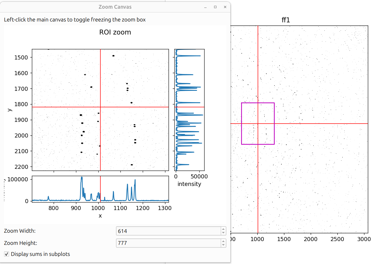
The zoom dialog shows:

• ROI zoom (left): A magnified view of the area around the cursor, with a histogram of intensity values below it.
• Intensity Sums: pixel intensity sum plots across rows (right) and columns (bottom)
• Zoom Width / Height: Controls the size of the zoom region in pixels.

Left-click the main canvas to toggle freezing the zoom box in place.

Stitching Raw Images

It is common in HEXRDGUI to take into account misalignments between subpanels by treating them as separate detectors. By default, visualizing the images in the raw view will display all subpanel images separately, like so:

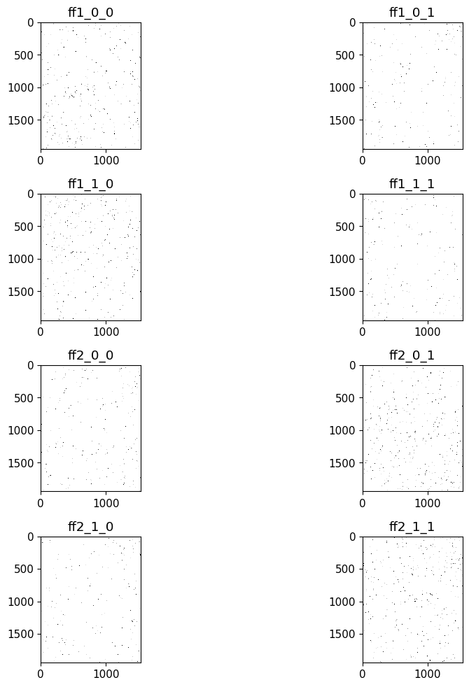
However, it can be helpful to view all subpanel images "stitched" into a larger, single detector image, as if the detector were perfectly flat. This is often the same as the image that the detector software outputs itself.

To do this, the instrument configuration must have a group defined for each subpanel. The groups should be the name of the detector that each subpanel is a part of (for instance, ff1_0_0 and ff1_0_1 are both subpanels for detector ff1, so the group should be ff1).

Additionally, each detector must have an roi specified under the pixels category that identifies the start pixels of the subpanel region. For example, roi: [0, 1536] means that the subpanel region starts at pixel 0 in i and 1536 in j. The end pixels of the region are determined automatically from the rows and columns.

If the group and roi are defined for each detector, a checkbox will appear in the raw Image Mode that is labeled "Stitch ROI Images". If checked, the subpanel regions will be stitched together into larger images like so:

Note that projections onto the detectors such as overlays (powder, rotation series, etc.) still take into account any subpanel misalignment and adjust their coordinates on the stitched images accordingly.

Cartesian View

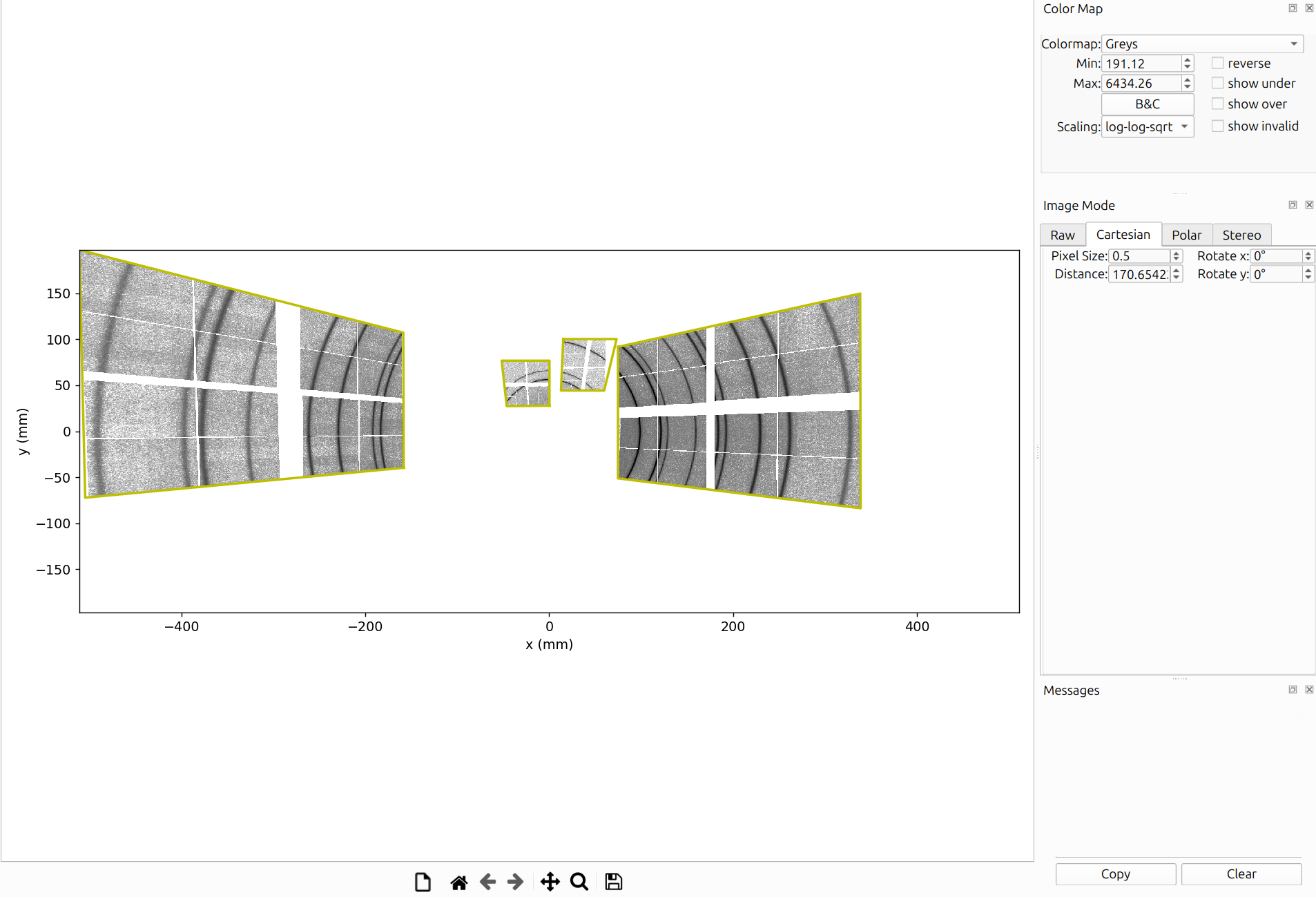
The Cartesian projection displays detector images in their real-space positions, as if you were at the sample looking out at the detectors. The images are projected onto a virtual plane at a configurable distance. This is useful for seeing how data from multiple detectors joins together. Gaps and overlaps between detectors become immediately apparent, and powder diffraction rings appear as smooth curves across the full angular range.

Cartesian View Options

• Pixel Size: The pixel size in mm for the virtual projection plane. Smaller values produce higher resolution but take longer to generate.
• Distance: The distance from the X-ray source to the virtual projection plane.
• Rotate x / Rotate y: Rotate the virtual plane normal around the X or Y axis. This tilts the virtual plane for different projection angles.

Polar View

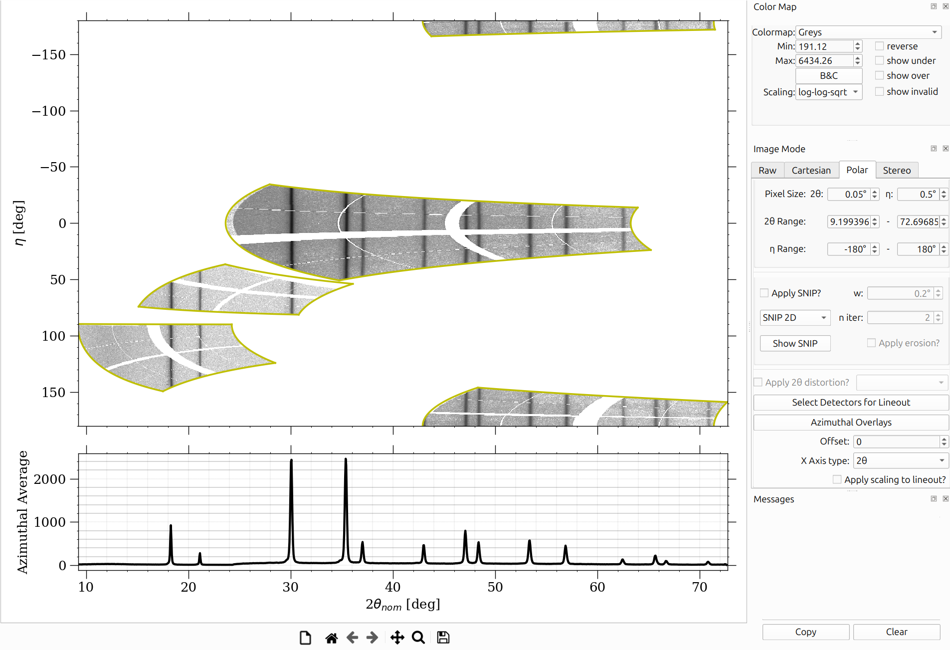
The Polar projection maps detector images into 2θ vs. η coordinates. In this view, powder diffraction (Debye-Scherrer) rings appear as vertical straight lines, making it easy to assess alignment and calibration quality. This is the primary view for powder calibration workflows (Fast Powder, Structureless) and WPPF.

An azimuthal lineout (integrated intensity vs. 2θ) is displayed below the main polar image.

Polar View Options

Pixel Size:

• 2θ: Angular resolution in the 2θ direction. Smaller values produce higher resolution but take longer to generate.
• η: Angular resolution in the η (azimuthal) direction. Smaller values produce higher resolution but take longer to generate.

Range:

• 2θ Range: The minimum and maximum 2θ angles displayed.
• η Range: The minimum and maximum η angles displayed. The min and max are synchronized to maintain a maximum span of 360 degrees.

SNIP Background Subtraction:

• Apply SNIP?: Enable SNIP (Statistics-sensitive Non-linear Iterative Peak-clipping) background subtraction.
• Algorithm: Choose between "Fast SNIP 1D", "SNIP 1D", or "SNIP 2D".
• w: Width parameter for the SNIP algorithm.
• n iter: Number of iterations for the SNIP algorithm.
• Show SNIP: Display the SNIP background subtraction result.
• Apply erosion?: Apply binary erosion to eliminate edge artifacts in the SNIP result.

2θ Distortion:

• Apply 2θ distortion?: Apply 2θ distortion correction from an overlay that has Pinhole Camera Distortion enabled.
• Overlay dropdown: Select which overlay to use for the distortion correction.

Lineout and Axis Options:

• Select Detectors for Lineout: Choose which detectors to include in the azimuthal lineout.
• Azimuthal Overlays: Open a manager for azimuthal overlay settings on the lineout plot.
• Offset: Rotate azimuthal overlays by this amount.
• X Axis type: Choose the x-axis units: "2θ" (degrees) or "Q" (inverse angstroms).
• Apply scaling to lineout?: When checked, the scaling from the color map is also applied to the lineout.

Other:

• Waterfall Plot: Create a waterfall plot from the image series. This generates a polar view image for every frame and stacks them. Only available when the image series has between 2 and 20 frames.

Switching Between X-Ray Sources

For instruments with multiple X-ray sources (2XRS configurations), a dropdown menu appears in the polar view options that allows you to switch which beam's projection is displayed. Each beam produces a different mapping from detector pixels to angular coordinates, so switching between sources shows how the data looks relative to each beam.

Stereographic View

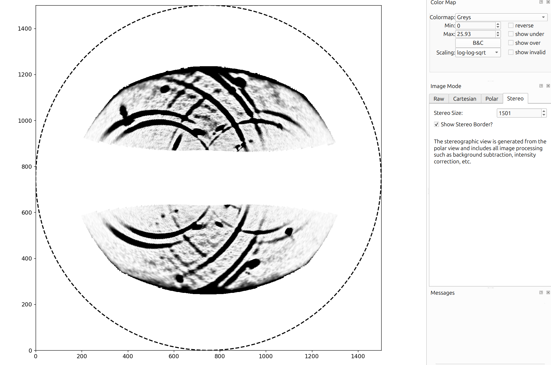
The Stereographic (Wulff) projection maps diffraction data onto a 2D stereographic circle. This view is useful for texture analysis and pole figure interpretation. Overlays are projected onto the stereographic circle alongside the data, allowing direct comparison of observed and simulated diffraction patterns.

Stereographic View Options

• Stereo Size: The number of pixels used for both width and height of the projection.
• Show Stereo Border?: Whether to draw the border around the valid stereographic region. Pixels beyond the border are NaN.

Unaggregated Image Series

When rotation series data is loaded, a toolbar appears at the bottom of the main canvas with controls for navigating individual frames.

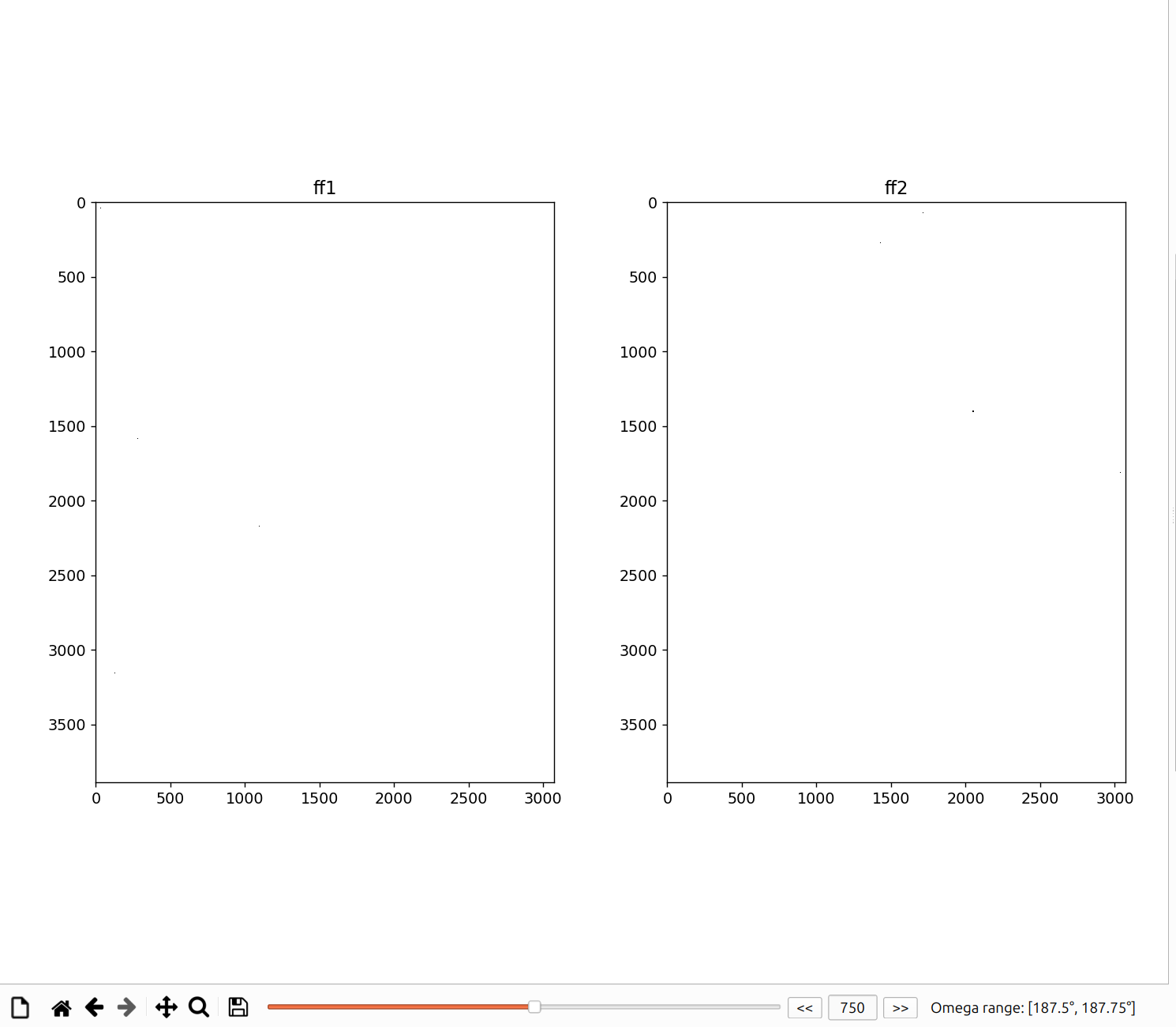
The toolbar includes:

• Slider: Drag to scrub through frames in the rotation series.
• Frame Number Editor: Type a specific frame number to jump directly to it.
• Back/Forward Buttons: Step through frames one at a time.
• Omega Range Display: Shows the omega rotation range corresponding to the current frame. The omega range is only displayed if the image series contains omega metadata.

This is essential for inspecting rotation series data frame-by-frame before running HEDM workflows. You can verify that spots appear and disappear at the expected omega angles, check for detector artifacts in individual frames, and ensure the omega values are set correctly.

Mouse Hover Information

When hovering the mouse over image data in any view, detailed crystallographic and spatial information is displayed at the bottom of the canvas.

The fields displayed depend on the view mode:

Raw, Cartesian, and Stereographic views:

• x, y: Pixel coordinates on the detector (raw) or virtual plane (Cartesian/Stereo).
• value: The pixel intensity at the cursor position.
• tth: Two-theta (2θ) scattering angle in degrees.
• eta: Azimuthal angle (η) in degrees.
• dsp: d-spacing in angstroms, computed from 2θ and the beam wavelength.
• chi: Angle between the diffraction plane normal (g-vector) and the sample normal.
• Q: Magnitude of the scattering vector in inverse angstroms, computed from 2θ and the beam energy.
• hkl: Miller indices of planes at this 2θ for the active material.
• detector: The detector name (shown when multiple detectors are present).

Polar view:

• tth: Two-theta angle in degrees (from the x-axis).
• eta: Azimuthal angle in degrees (from the y-axis).
• value: Pixel intensity at the cursor position.
• dsp, chi, Q, hkl: Same as above.
• detector: The detector name (shown when multiple detectors are present).

When hovering over the azimuthal lineout plot (below the main polar image), only tth, intensity, and Q are shown.

Color Map

The color map editor controls how image intensities are mapped to colors.

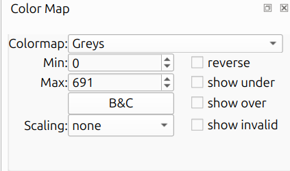
• Colormap: The matplotlib colormap used for display (e.g., Greys, viridis, plasma).
• Min / Max: The data range for color mapping. Values at or below Min map to the bottom of the colormap; values at or above Max map to the top. These are auto-populated based on percentile analysis of the data.
• B&C: Opens the Brightness & Contrast editor (inspired by the one in ImageJ). See Brightness & Contrast Editor below.
• Scaling: Applies a mathematical transformation to the data before colormap application. Options are:
  • none: No transformation (raw values).
  • sqrt: Square root scaling, useful for emphasizing lower values.
  • log: Logarithmic scaling, useful for compressing wide dynamic range.
  • log-log-sqrt: Extreme compression for very wide dynamic range.
• reverse: Inverts the colormap gradient.
• show under: Colors values below the minimum as blue.
• show over: Colors values above the maximum as red.
• show invalid: Colors invalid (NaN) pixels with a user-selected color. A color picker dialog appears when this is checked.

Brightness & Contrast Editor

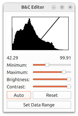
The Brightness & Contrast (B&C) editor, inspired by the one in ImageJ, provides an interactive way to adjust the color mapping range. At the top is a histogram of the image data, with a diagonal line indicating the current mapping from intensity values to display colors. The numbers below the histogram show the current minimum and maximum values.

• Minimum / Maximum: Sliders to adjust the lower and upper bounds of the color mapping range. These correspond to the Min / Max fields in the color map editor.
• Brightness: Shifts both the minimum and maximum together, making the overall image brighter or darker.
• Contrast: Adjusts the width of the mapping range. Higher contrast narrows the range, making differences in intensity more visible.
• Auto: Automatically sets the minimum and maximum based on percentile analysis of the image data.
• Reset: Restores the minimum and maximum to the full data range.
• Set Data Range: Sets the minimum and maximum to the absolute minimum and maximum values in the image data.