Rotation Series (ff-HEDM)

Rotation Series calibration is designed for refining detector positions and grain parameters using far-field HEDM (High Energy Diffraction Microscopy) data. It works in three main steps:

1. Configure: Select grains and set Pull Spots options.
2. Pull Spots: Measure actual diffraction spot locations from the rotation series data.
3. Calibration: Refine parameters in the calibration dialog to minimize the residual between measured and predicted spot positions.

Prerequisites

Before running Rotation Series calibration, you must have:

1. Loaded rotation series image data (see Rotation Series Data).
2. Completed HEDM indexing and Fit Grains (a grains table must exist from these steps), or a grains.out file containing a pre-determined grains table.
3. The instrument configuration should be reasonably close to correct already (can be off by the eta, tth, and omega tolerances specified). This is necessary for Pull Spots to be able to correctly pair spots in the data with grains and their HKLs. You can visually inspect the data in the different views with the rotation series overlay displayed (see the Selecting Grains section for generating these) to determine if the actual spot data lies within the rotation series bounding boxes.

Navigate to Run -> Calibration -> Rotation Series (ff-HEDM) from the menu bar to begin.

Step 1: HEDM Calibration Options

The first dialog configures the Pull Spots options, which control how measured spot locations are extracted from the rotation series data and paired with specific grains and HKLs.

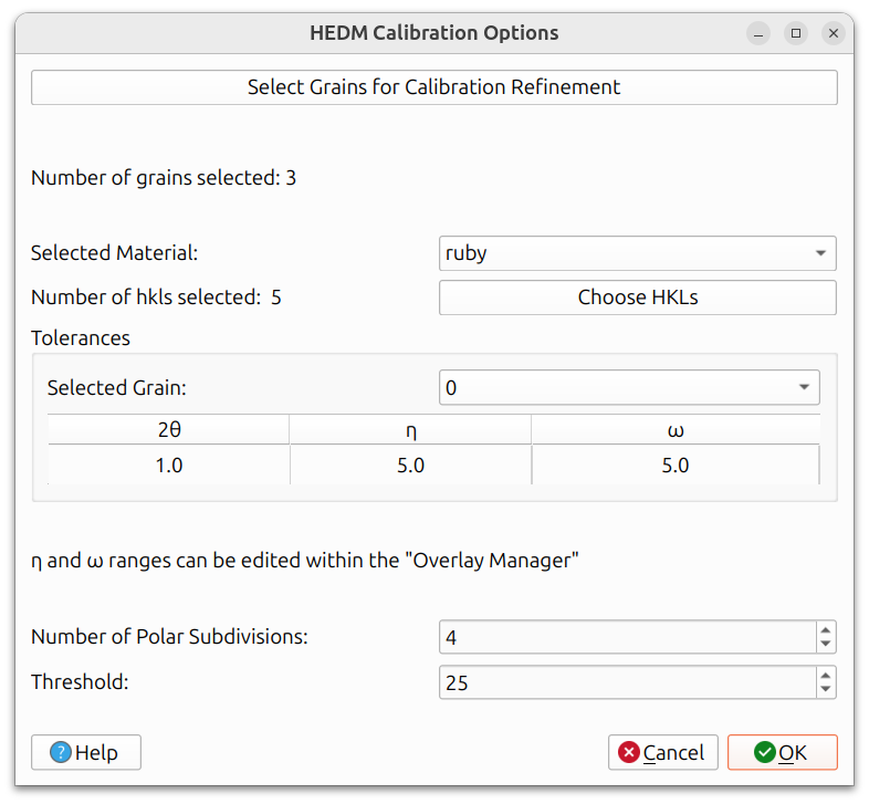
Selecting Grains

Click "Select Grains for Calibration Refinement" to choose which grains from the grains table will be used. You do not need to use all grains; oftentimes one well-characterized grain is sufficient, but multiple grains can optionally be used.

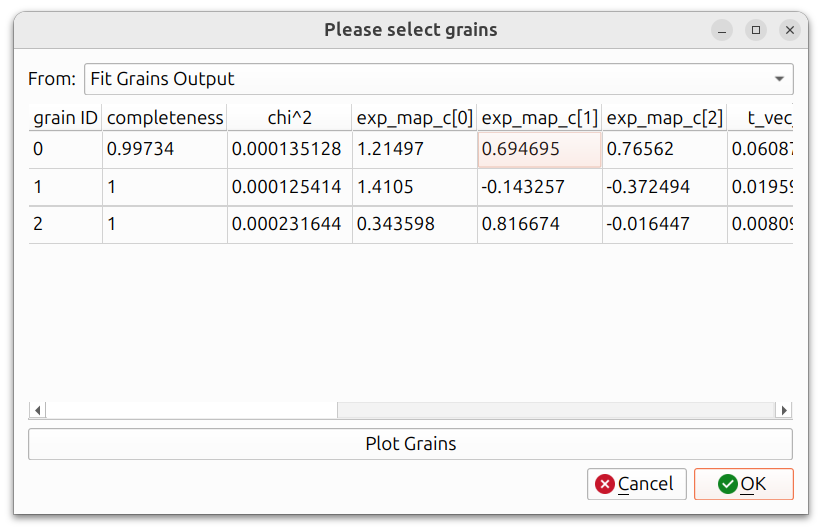
The "From" dropdown provides several sources for loading grains: "HEDM Calibration Output" (a previous calibration in the current session), "Fit Grains Output" (a previous fit-grains run in the current session), "Find Orientations Output" (a previous find-orientations run in the current session), or "File", where they are loaded from a grains.out file.

After clicking OK, rotation series overlays are automatically created for the selected grains. You can inspect these overlays in the main canvas to verify that the predicted spot positions look reasonable.

Important: Check that the 2θ and η widths of the rotation series overlays surround most of the observed spots. These tolerances determine which spots will be included when Pull Spots runs. If the tolerances are too narrow, spots will be missed; if too wide, noise or neighboring spots may be included.

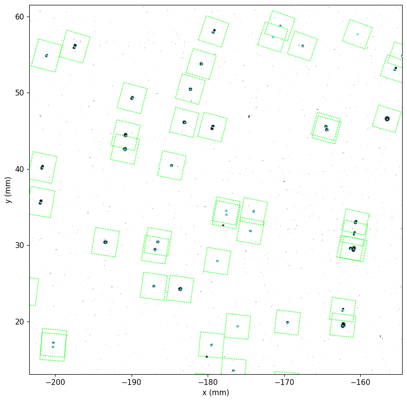
The above image shows a zoomed in region of the Cartesian view, where the image data was aggregated over all omega frames using "Maximum" aggregation. It includes the data (black spots in the background), the rotation series overlays (cyan dots on top of the spot data), and green rectangles (bounding boxes for the eta and two theta widths).

Pull Spots Options

Once you are satisfied that the overlays cover the relevant spots, proceed to check the remaining options. These settings control how spot data is pulled from the image data and paired with specific grains and HKLs.

• Selected Material: The material to use for calibration.
• Choose HKLs: Select which HKL reflections to include.
• Tolerances: The 2θ, η, and ω widths that define the search windows around each predicted spot. These can be set per grain. The η and ω ranges can also be edited within the Overlay Manager.
• Number of Polar Subdivisions: Controls the angular resolution when extracting spot intensities.
• Threshold: The minimum intensity threshold for including a spot.

Step 2: Pull Spots

Once you are satisfied with all Pull Spots options, click OK to run Pull Spots. This extracts the measured spot locations from the rotation series image data by searching within the tolerance windows defined by the overlays.

This step may take some time depending on the size of the dataset and the number of grains selected.

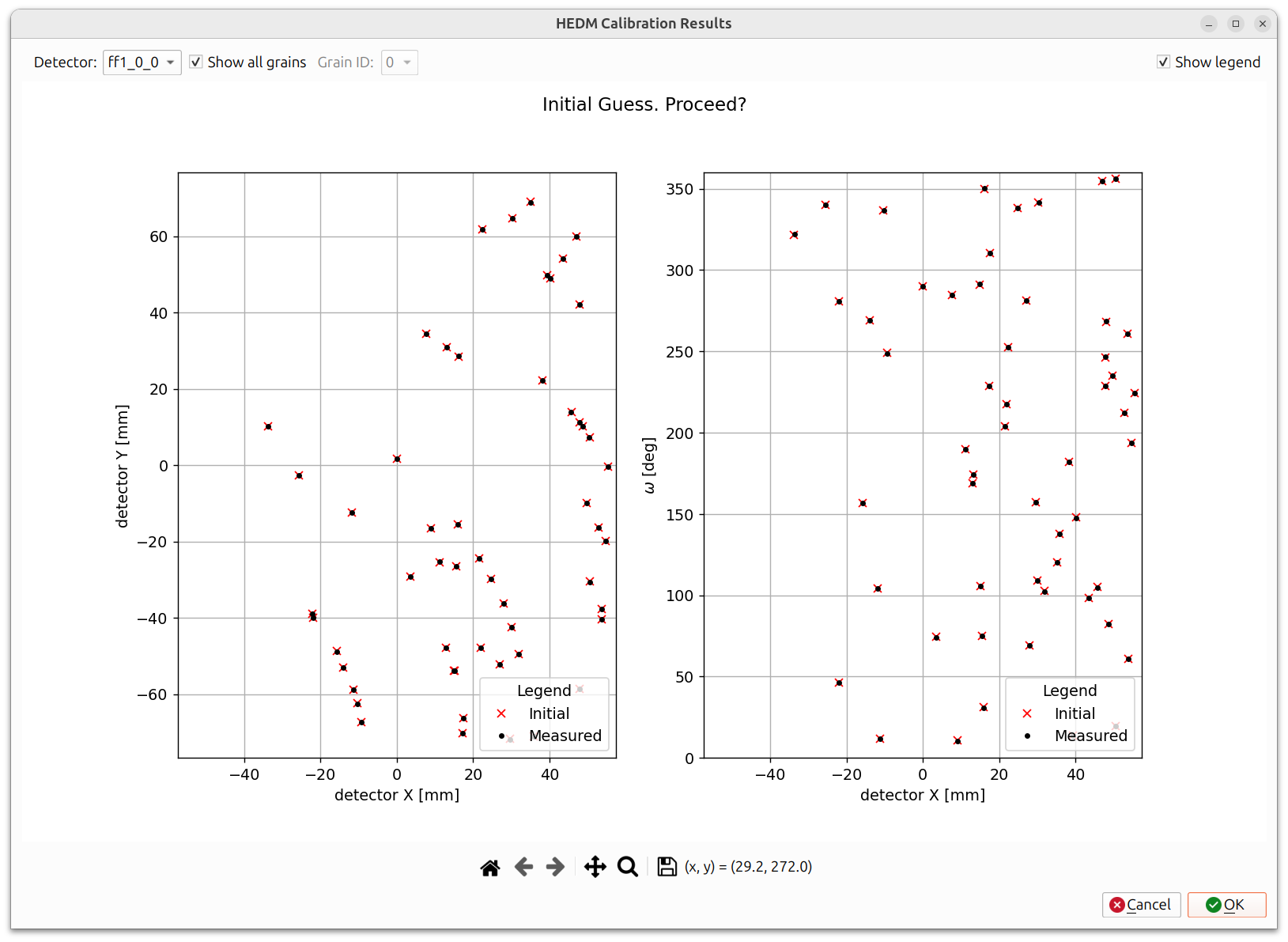
HEDM Calibration Results Dialog

After Pull Spots completes, a results dialog appears showing the measured spot positions (black dots) overlaid with the initial predicted positions (red x's). Two plots are shown: the left plot shows detector X vs. detector Y positions, and the right plot shows detector X vs. ω positions. You can filter by detector and grain ID using the dropdowns at the top.

Inspect this carefully:

• If the measured and predicted positions align well, click OK to proceed to the calibration dialog.
• If they do not look good, click Cancel and go back to adjust your tolerances, grain selection, or other parameters before trying again.

Step 3: Calibration Dialog

After accepting the pull spots results, the calibration dialog appears.

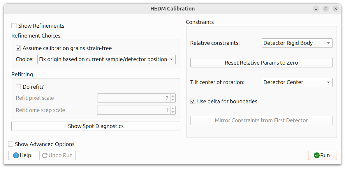
Refinement Choices

The "Refinement Choices" section at the top of the dialog provides options for how the calibration handles the origin and strain:

• Assume calibration grains strain-free: When checked, sets all calibration grains' stretch tensors to identity and holds them fixed during refinement.
• Fix origin based on current sample/detector position: Holds detectors fixed along the Y axis during refinement.
• Reset origin to grain centroid position: Sets the first calibration grain's centroid to [0,0,0] and holds it fixed during refinement.
• Reset Y axis origin to grain's Y position: Sets the first calibration grain's Y position to zero and holds it fixed in Y during refinement.
• Custom refinement parameters: Uses the current parameter refinement choices as-is. Warning: incompatible choices can be made without proper consideration of the system's degrees of freedom.

The parameter tree view is hidden by default; check "Show Refinements" to reveal it. As the "Refinement Choices" setting is changed, you can view which parameters are automatically modified in the tree view.

Manually modifying which parameters are marked for refinement will automatically switch the choice to "Custom refinement parameters". This is only recommended for advanced users.

Refitting

The "Refitting" section controls whether a second refinement pass is performed after filtering out outlier reflections:

• Do refit?: When checked, the grain and instrument parameters are first refined, then reflections too far from predicted values are filtered out, and the parameters are refined again. When unchecked, only a single refinement pass is performed.
• Refit pixel scale: The maximum distance (in pixels) in x or y before a reflection is filtered out during the refit step.
• Refit ome step scale: The maximum distance in omega steps before a reflection is filtered out. For example, if the omega step size is 0.25 degrees and this value is 2, reflections more than 0.5 degrees away in omega are filtered.

Spot Diagnostics

The "Show Spot Diagnostics" button opens a dialog for visualizing the residuals between predicted and measured spot positions. This is useful for evaluating calibration quality and identifying problematic spots or detectors.

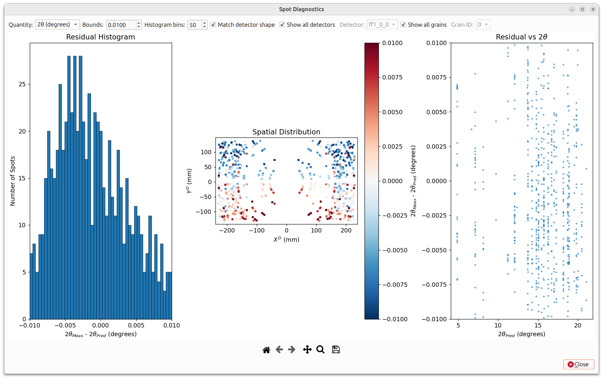
The dialog displays three plots:

• Residual Histogram (left): A histogram of the residuals (measured - predicted) for the selected quantity. This gives an overall view of the residual distribution. A well-calibrated instrument should show a narrow, symmetric distribution centered near zero.
• Spatial Distribution (center): A scatter plot showing the residuals at each spot's position on the detector, color-coded by residual magnitude (using a red-blue colormap). This helps identify whether residuals are spatially correlated, which could indicate systematic detector misalignment.
• Residual vs Predicted Value (right): A scatter plot of residuals versus the predicted value of the selected quantity. This helps reveal trends, such as residuals that grow at higher 2θ angles.

The following controls are available along the top of the dialog:

• Quantity: The quantity to analyze. Options include 2θ, η, ω, X, and Y. Each has different default bounds.
• Bounds: The symmetric range for the histogram and color scale. Adjusting this focuses the view on residuals within the specified range.
• Histogram bins: The number of bins in the residual histogram.
• Match detector shape: When checked, the spatial distribution plot is scaled to match the physical detector dimensions.
• Show all detectors / Detector: Filter by a specific detector or show all detectors combined.
• Show all grains / Grain ID: Filter by a specific grain or show all grains combined.

If the Spot Diagnostics dialog is open during calibration, it automatically updates after each calibration run, so you can observe how the residuals change as parameters are refined.

This dialog is also available from the Fit Grains Results dialog, where it can be used to evaluate spot quality before calibration.

Refinable Parameters

When "Show Refinements" is checked, the tree view includes:

• Instrument parameters: Detector tilts, translations, beam energy, beam vector, etc.
• Grain parameters (per grain):
  • Orientation: parameters describing the crystal orientation.
  • Position: The grain's position in the sample frame.
  • Stretch Matrix: The symmetric stretch tensor, encoding lattice strain.

See General Calibration Information for details on constraints, delta boundaries, and advanced optimizer options.

Running and Undoing

Click Run to execute the calibration. Parameters marked with "Vary" will be refined to minimize the residual between measured and predicted spot locations. Click Undo Run to revert if needed. A full undo stack is maintained.

After running, a results dialog appears showing the initial predicted positions (red x's), measured positions (black dots), and final predicted positions after calibration (blue +'s). If the calibration improved the fit, the blue markers should be closer to the black dots than the red markers are.

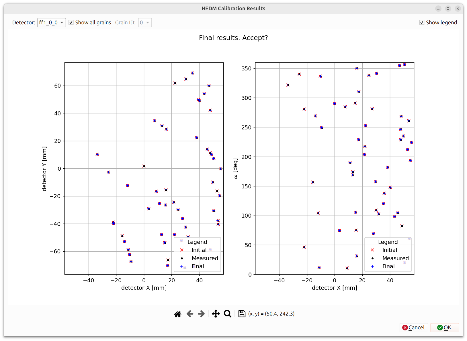
As with other calibrations, an iterative approach is recommended. Use the refinement choices as a starting point, run, inspect results, then adjust as needed.

When you are satisfied with the results, close the dialog to finish.